Modelling, Simulation and Control of Hydro-Power System - Part 2
Theoretical model of the lakes
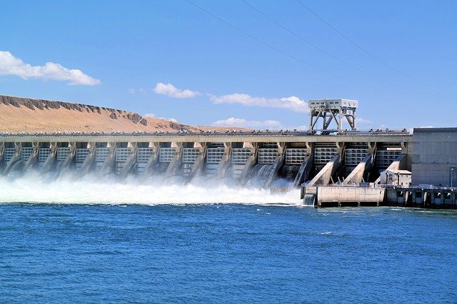
 Image by Russ McElroy from Pixabay
Overview
In the previous post of this series (see here), I showed an overview of the system we intend to model and investigate. In this post I will show how to develop a simple yet effective mathematical representation of the series of lakes in the hydro-power system.
The main use of these lakes is to work as a battery, i.e energy storage. At times when energy is at low demand, water can be pumped from the river to the lakes and stored there as potential energy. When there is a greater demand and only the level of water from the river can not provide enough energy, water can flow from the lakes to the river through turbines, using its kinetic energy to generate extra energy. Notice that this process is, in a real-world case, not 100% efficient. This means that more energy is needed to pump the water from the river to the lakes, then can be extracted by turbining from the lakes to the river. Yet, it can be a useful technique to keep the balance in energy generation, and also to redirect volume of water when its excess can cause floods downstream.
Without further delay, let’s start the modeling process.
Mathematical representation of the lakes
The water stored in the lake changes according the inflow and outflow rates. As the volume of water decreases, the level also decreases. In essence the mass conservation is the basic equation to describe the lakes:
Where
Where
The above equation is an ordinary differential equation, relating the rate of change of volume (
Power generated/consumed by pumps and turbines
The power
Where
Pipes and valves
The connection between lake 1 and 2 is made through a valve. The discharge through this element can in general be modelled by a non-linear relationship with the difference in height upstream and downstream
Where
Analytical solution of lake storage with sinusoidal inflow and constant outflow (pump)
It is always useful to have some analytical solution of ODE problems to compare how good are numerical solutions obtained in a later step. Coming back to the mass conservation:
Let’s consider a very simple lake in the form of a cube. Thus, the cross section area is constant.
The equation simplifies to:
Say the outlet is regulated by a pump, with a constant flow rate of
Call
Integrate it.
Which gives us the general solution to this problem. Now let’s fix some numerical values for simulation.
Apply initial condition
The final analytical solution is,
The equation above is used to calculate the water level profile of the lake for any time

Another analytical solution, with variable cross-section
Let’s perform a similar analysis, as the one shown above, but now using a lake which has a variable cross-section area. Say that the cross-section area follows the pattern below:
Where
Integrate it.
Which gives us the general solution to this problem. Now let’s fix some numerical values for simulation.
Apply initial condition
Therefore the specific solution is,
Substituting the values here we find that,
The final analytical solution is,
The equation above is used to calculate the water level profile of the lake for any time

In the next post, we will see how to model the reaches using the De Saint Venant Equations. I see you in the next post.